 github
Tutorial 1: Bregman soft clustering
This tutorial reports the experiment proposed by Banerjee et al. in [5].
We create three 1-dimensional datasets of 1000 sample each, based on mixture models
of Gaussian, Poisson and Binomial distributions, respectively. All the mixture models had three
components with means centered at 10, 20 and 40, respectively. The standard deviation s of
the Gaussian densities was set to 5 and the number of trials N of the Binomial distribution was set
to 100 so as to make the three models somewhat similar to each other, in the sense that the variance
is approximately the same for all three models.
For each dataset, we estimate the parameters of three mixture models of Gaussian, Poisson and Binomial
distributions using the proposed Bregman soft clustering implementation.
The quality of the clustering was measured in terms of the normalized mutual information (Strehl and Ghosh, 2002)
between the predicted clusters and original clusters (based on the actual generating mixture component).
The results were averaged over 100 trials.
This tutorial is available on github.
Tutorial 2: Parameter estimation of a mixture of Gaussian
This tutorial consists in the following steps:
- We define a mixture f of univariate Gaussians of n components (e.g. n=3).
- We draw m points from f (e.g. m=1000).
- We estimate the parameters of a mixture f1 of univariate Gaussians of n components using a classical expectation-maximization (EM) algorithm.
- We estimate the parameters of a mixture f2 of univariate Gaussians of n components using the Bregman soft clustering implementation (based on the duality of regular exponential families with regular Bregman divergences).
We then check that the estimated mixtures f1 and f2 are similar.
This tutorial is available on github.
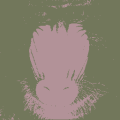
Tutorial 3: Mixture model simplification
This tutorial consists in the following steps:
- Read an image file.
- Load the correponding mixture of Gaussians (depending on the image and on the desired number number of components n) from a file. If the mixture doesn't exist yet, the mixture is estimated from the pixels of the image using Bregman soft clustering, and the mixture is saved in an output file.
- Compute the image segmentation from the initial mixture model and save the segmentation result in an output file.
- Simplify the mixture model in a mixture of m components.
- Compute the corresponding image segmentation and save the segmentation result in an output file.
This tutorial is available on github.
 |
 |
 |
 |
 |
 |
| m=1 | m=2 | m=4 | m=8 | m=16 | m=32 |
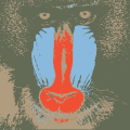
Tutorial 4: Hierarchical mixture models
This tutorial consists in the following steps:
- Read an image file.
- Load the correponding mixture of Gaussians (depending on the image and on the desired number of components n) from a file. If the mixture doesn't exist yet, the mixture is estimated from the RGB pixels of the image using Bregman soft clustering, and the mixture is saved in an output file.
- Compute the image segmentation from the initial mixture model and save the segmentation in an output file.
- Compute a hierachical mixture model from the initial mixture model.
- Extract a simpler mixture model of m components from the hierachical mixture model.
- Compute the corresponding image segmentation and save the segmentation result in an output file.
Note that the hierachical mixture model allows to automatically extract the optimal number of components in the mixture model.
To do this, use the method getOptimalMixtureModel(t) instead of getPrecision(m) in the tutorial.
This tutorial is available on github.
 |
 |
 |
 |
 |
 |
| m=1 | m=2 | m=4 | m=8 | m=16 | m=32 |
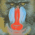
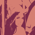
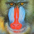
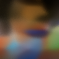
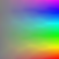
Tutorial 5: Statistical images
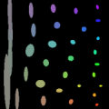
For this tutorial, we consider an input image as a set of pixels in a 5-dimensional space (color information RGB + position information XY). The mixture of Gaussians f is learnt from the set of pixels using the Bregman soft clustering algorithm. Then, we create two images (see Fig.3):
- Each Gaussian is represented by an ellipse illustrating the mean (color + position) and the variance-covariance matrix (ellipse shape) (see row 2, Fig. 3).
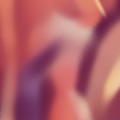
- Draw random points from f until at least 20 points per pixels have been drawn. Then, the color value of the statistical image pixel at the position (X,Y) is the average color value of the drawn points at the same position (see row 3, Fig. 3).
The proposed tutorial shows that the image structure can be captured into a mixture of Gaussians. The image is then represented by a small
set of parameters (in comparison to the number of pixels) which is well adapted to applications such as color image retrieval. Considering an
input image represented by its mixture of Gaussians, it is then trivial to retrieve, in a image database, a set of images have a similar color organization.
This tutorial is available on github.
| Original images |
 |
 |
 |
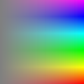 |
| Gaussian representation |
 |
 |
 |
 |
| Statistical images |
 |
 |
 |
 |